In this blog post, we delve into the nitty-gritty of the RPC camera model. We explore the underlying motivations behind its development, discuss its applications, and provide practical insights into effectively utilizing it.
The logic behind it
RPC, also known as the Rational Polynomial Camera model, is widely recognized as a standard approach in satellite imagery for addressing the challenge of multiple camera models. In some contexts, it is referred to as RFM, which stands for Rational Function Model. The primary purpose of this model is to provide a unified framework that facilitates seamless communication between various stakeholders.
The motivation behind developing the RPC model stems from the existence of numerous camera models, each with its unique mathematical representation. Instead of accommodating each model, the RPC model serves as a comprehensive solution capable of describing the majority of optical configurations and sensors. This simplifies the process for end users, enabling them to work with a single model that encompasses a wide range of camera variations.
Let’s begin our introduction to the RPC model by starting from the basics. We’ll initially explore the pinhole model, which provides a simplified representation of a camera, and then we’ll expand upon this concept to develop a more comprehensive camera model. Ultimately, we’ll describe both models using an RPC function.
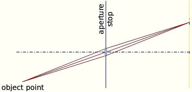
In the pinhole model, all light rays are assumed to travel in straight lines along both axes. In real life, light rays will strictly travel in a straight line and will never travel in curves our rays can, so from this point on the rays will no longer be strictly speaking light rays. This model defines a focal length that can be visualized as a constant angle, denoted as alpha, over which the entire image is spread. Consequently, in our image grid, the starting pixel (0) corresponds to a ray with an angle of -[alpha], and the ending pixel (W) corresponds to a ray with an angle of [alpha]. The image center, typically located at H/2, W/2, is assigned an angle of 0.
As we progress to a more complex camera model, we need to consider lens distortion. Unlike the previous linear angle relationship in the pinhole model, this distortion model introduces non-linearity. Consequently, the angle shift between two grid points, such as 100 and 101, is no longer the same as between 500 and 501. Each ray now has a distinct angle based on its location, resulting in a distorted image. To account for this, we need to define a function that relates the angle to the distance from the image center (H/2, W/2).
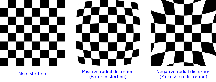
One commonly used distortion model is the Brown-Conrady distortion model, which is defined as follows:
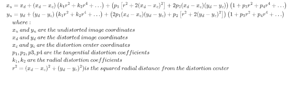
In this model, the angle is a function of the position on the image grid and can vary at each point. Allowing a governed flexibility based on model constraints.
For more detail on pinhole model and camera distortion: https://ori.codes/artificial-intelligence/camera-calibration/camera-distortions/
From a satellite perspective, our goal is to establish a mapping between the image grid, or each pixel, and its corresponding rays (and where it will hit the Earth) in a way that can be universally applied to different camera models. This mapping should allow us to determine the location on the planet based on the trajectory of these rays.
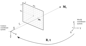
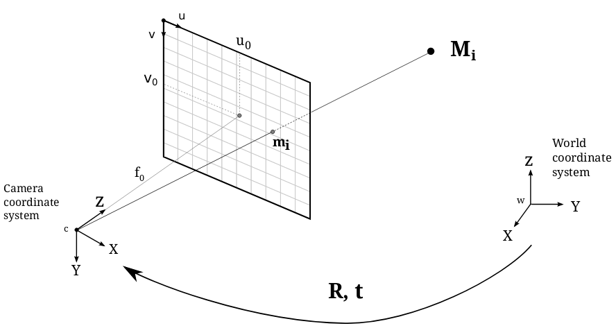
In the pinhole model, the linear projection mapping is derived from the camera’s position relative to the world. By projecting the rays from the camera’s location, they extend until they intersect with the surface of the Earth. This linear projection enables us to determine the location on the planet corresponding to each pixel in the image grid. As can be seen in the figure below
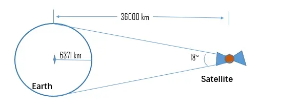
When considering the perspective of rays, each ray is projected to a different location based on the altitude of the object it encounters. The object’s location determines where the ray will intersect with the Earth’s surface. If we examine it from the ground’s perspective, each triplet [x, y, z] on the ground can be mapped to the camera plane coordinates [u, v] based on the location where the ray intersects the camera plane. This two-way transformation establishes a correspondence between every point on the world map and its corresponding pixel value, as well as assigning a 3D coordinate to each unit in the grid.
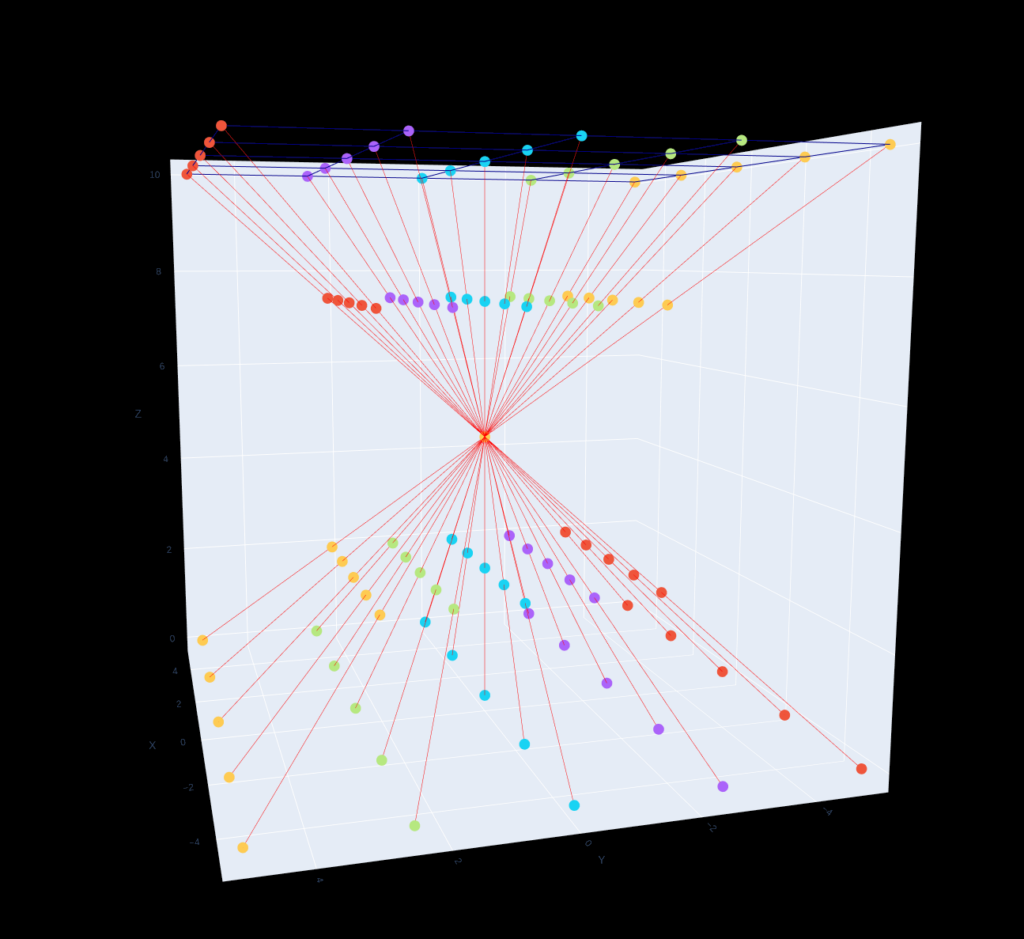
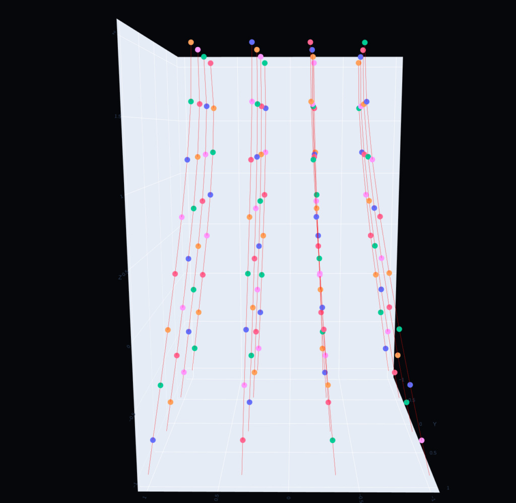
To illustrate this mapping, let’s create a visual representation of the RPC model using a simulated pinhole camera on a satellite. In this example, we depict the travel path of rays from the camera plane to various locations on the ground. In the simple pinhole case, where the lines are linear, the top of the visual represents the assumed camera plane, while the bottom represents its mapping onto the ground. The lines appear straight and linear, adhering to the pinhole camera model, and the angle is determined by the focal length, representing the angle of the rays.
Similarly, in the case of a distortion lens, we can visualize a similar image. However, the distortion, in this case, is caused by a shift in the angle only around the lens itself. Each ray departing from the lens follows a different angle compared to its neighboring ray. Unlike the simple linear lines in the pinhole model, the rational polynomial definition used in the RPC model allows for the depiction of multiple curves, not limited to a single kink in the ray line. This flexibility is showcased in the image below:
Constructing the RPC
To establish the formulation of the RPC model, our objective is to create a mapping between a point in the world, specified by latitude, longitude, and altitude, and its corresponding position on the image plane, represented by coordinates (u, v).
Given that the world is vast and even the largest captured image covers only a portion of it, it is more convenient to work with a normalized coordinate system rather than an actual coordinate system. Both the image and the world coordinate will be defined within the extent of [-1, 1].
For instance, if our image size is 1920×1080 pixels, we can begin the normalization process by shifting the image to the middle. This means subtracting 960 from the width (1920) and 540 from the height (1080), resulting in a coordinate range of [-540, 540] for both dimensions. The next step is to normalize these coordinates by dividing them by the shifted width and height values (960 and 540, respectively). This normalization process ensures that the final coordinate range is [-1, 1].
In our three-dimensional world, we follow a similar normalization process for all three axes (X, Y, Z) or (latitude, longitude, altitude). However, defining the center of the world becomes slightly more flexible. Typically, we define the center to be the projected ray originating from the middle pixel in the image coordinates, which corresponds to [0, 0] in the normalized coordinates or [960, 540] in the actual image coordinates.
For altitude normalization, we have a couple of options. One approach is to bind the altitude to a predefined range based on the available altitude information in the target frame. Another approach is to place the altitude scale in the middle by considering the highest and lowest points on the globe, effectively accommodating any altitude measurements in between. However, it’s important to note that this method may result in some loss of measurement accuracy.
Therefore, the RPC camera model includes normalization constants to transform the image from its actual coordinate system and the world coordinates to a normalized coordinate set. These constants ensure consistency between the different coordinate systems.
For example
LINE_OFF: 539.5
SAMP_OFF: 1279.5
LAT_OFF: -14.0539237813539
LONG_OFF: -72.2617603159834
HEIGHT_OFF: 3500
LINE_SCALE: 540.5
SAMP_SCALE: 1280.5
LAT_SCALE: 0.0125517537538986
LONG_SCALE: 0.0131980971833769
_SCALE: 8000
where the offset (_OFF) and scale (_SCALE) factors for each of the following parameters: altitude [HEIGHT], Line[row], SAMP [col], LAT [latitude], LONG [longitude]. These factors will define the adjustment and scale to actual world values.
Apart from normalization, the RPC model is defined as a rational function, specifically a third-degree polynomial divided by another third-degree polynomial. This rational function provides a mathematical representation of the mapping between the normalized image coordinates and the corresponding world coordinates. The polynomial terms in the numerator and denominator capture the non-linear characteristics of the mapping, allowing for accurate transformations between the image and world spaces.
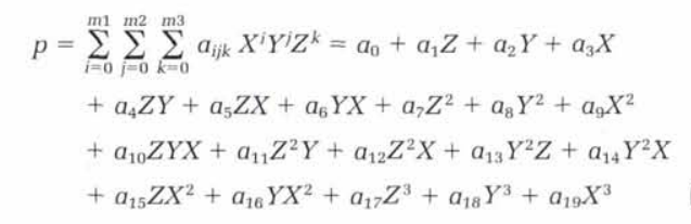
In the RPC model, the mapping from latitude (LAT), longitude (LONG), and altitude (ALT) to image row (r) and column (c) coordinates involves four third-degree polynomials, split into two pairs for rows and columns separately.
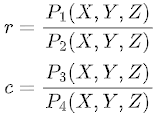
The mapping for rows can be expressed as r = p1/p2, and the mapping for columns as c = p3/p4. Here, p1, p2, p3, and p4 are the polynomials defined for the numerator and denominator of both row and column mappings.
Each polynomial function consists of three variables: X, Y, and Z, representing the normalized latitude, longitude, and altitude, respectively.
Expanding this form results in a total of 20 coefficients indexed 0-19 for each polynomial. However, it is important to note that the first coefficient of the denominator polynomial is always set to 1. Therefore, the RPC model has a total of 78 parameters (20 + 20 + 19 + 19) that define the transformation for a given image.
Applying the model to an image
To apply the RPC model to an image, let’s consider a simple example. We will assume that we want to project our image onto the world using the RPC model. The desired size of the final world image is [100×100].
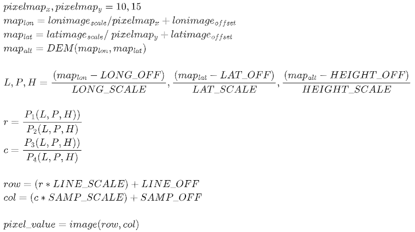
First, we need to read the RPC header file to determine the location on Earth we are interested in. This information is typically provided through the lat/lon _off parameters. We will also obtain the image size (100×100) and the scale from the header to determine the grid size for the image in terms of latitude and longitude, which will be lat_scale/100 and lon_scale/100.
However, we still need the altitude information. It can be either a single altitude level (e.g., 0) or derived from the actual terrain in the area using a Digital Elevation Model (DEM) file. The DEM file provides altitude values (H) for each x, y coordinate with a certain resolution.
Once we have all the necessary information, we can apply the RPC model to each element in our grid. Let’s assume we select a sample in the middle of the grid [10,15]. We will color the value of that pixel in the grid (x, y, z) by first normalizing it, by getting the location (lat,lon) and alt from the dem in lat,lon coordinate of the center pixel in with the corresponding data and then applying the polynomial and division operations. Finally, we will rescale the result (r,c) and will get an image coordinate to sample from one image space to the desired range. so formally here we will get
The official coefficient assignment order, defined in http://geotiff.maptools.org/rpc_prop.html is
But can it be derived?
Recent advances in Multi-View Stereo (MVS) techniques have highlighted the need for a differentiable formulation of the RPC model to enable gradient propagation. The paper titled “Rational Polynomial Camera Model Warping for Deep Learning Based Satellite Multi-View Stereo Matching” suggests formulating the problem using a quaternion cubic homogeneous polynomial or a quaternion-based tensor, where the multiplication operation yields the application of the RPC model.
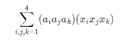
This quaternion-based tensor consists of a 4x4x4 tensor (64 elements) to be derived from the 20 polynomial coefficients of a single mapping. The transformation needs to be adjusted during the construction of the tensor according to the specific form. In the referenced article, the tensor construction is described as T[i][j][k] = ai * aj * ak, and the polynomial function P(X, Y, Z) = ΣΣΣcijk * Xi * Yj * Zk translates to the multiplication of quaternion elements, ai * aj * ak, in the sum.
Therefore, the 3D tensor transformation derived from the RPC coefficients corresponds to the mapping described in the paper using the formulated quaternion-based tensor.
ndeed, in the construction of the tensor, the relationship between the 64 tensor elements and the RPC coefficients is determined by the repeated use of the same coefficients. When multiplying by the vector in matrix multiplication form, it yields the same calculation as the conventional approach to computing the non-quaternion polynomial.
In the tensor construction, the indices of the tensor describe the power of each element, with the main diagonal representing the values for the power of 3 (x^3, y^3, z^3) and 0 for the initial index.
The second case in the tensor construction occurs when two indices are the same (i = j, j = k, i = k). Here, we observe that for each unique multiplier, there are 3 elements in the tensor. To ensure the same quality for these coefficients, they are divided by 3.
The last case involves elements where none of the indices are the same, resulting in 6 tensor elements representing the same polynomial multiplier. In this case, they are divided by 6 to maintain consistency.
This adjustment in the tensor construction helps ensure the proper relationship between the tensor elements and the RPC coefficients, allowing for accurate and consistent mapping between the quaternion-based tensor and the RPC model.
for example:
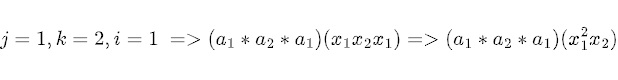
To account for the three permutations of indices (x_1, x_2), (x_2, x_1), and (x_1, x_2) again that result in the term x_1^2 * x_2, we need to divide the corresponding tensor elements by the repetition of unique numbers. This division ensures that the final summation is correct. Specifically, in this case, we divide by 3 to properly handle the three permutations.
Similarly, in cases where none of the indices are the same, resulting in terms like x_1 * x_2 * x_3, there are six permutations (x_1, x_2, x_3), (x_1, x_3, x_2), (x_2, x_1, x_3), (x_2, x_3, x_1), (x_3, x_1, x_2), and (x_3, x_2, x_1). Therefore, in the final summation, we divide the corresponding tensor elements by 6 to properly account for the repetition of unique numbers.
Which allows us to compute the RPC transform as
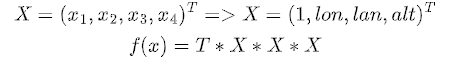
When multiplying the vectors X = (X_1, X_2, X_3) in the tensor construction, it will result in a 4×4 tensor. This tensor holds the possible powers of X in the normal form, with each element representing the corresponding power of X.
# a simple and not efficent example on creating the tensor just to drive the point clear
import torch
import numpy as np
coef = np.ones(20) # loaded RPC single poly coefficent
mapping = {
(0,0,0): 'c0',
(0,0,1): 'c1',
(0,0,2): 'c2',
(0,0,3): 'c3',
(0,1,0): 'c1',
(0,1,1): 'c7',
(0,1,2): 'c4',
(0,1,3): 'c5',
(0,2,0): 'c2',
(0,2,1): 'c4',
(0,2,2): 'c8',
(0,2,3): 'c6',
(0,3,0): 'c3',
(0,3,1): 'c5',
(0,3,2): 'c6',
(0,3,3): 'c9',
(1,0,0): 'c1',
(1,0,1): 'c7',
(1,0,2): 'c4',
(1,0,3): 'c5',
(1,1,0): 'c7',
(1,1,1): 'c11',
(1,1,2): 'c14',
(1,1,3): 'c17',
(1,2,0): 'c4',
(1,2,1): 'c14',
(1,2,2): 'c12',
(1,2,3): 'c10',
(1,3,0): 'c5',
(1,3,1): 'c17',
(1,3,2): 'c10',
(1,3,3): 'c13',
(2,0,0): 'c2',
(2,0,1): 'c4',
(2,0,2): 'c8',
(2,0,3): 'c6',
(2,1,0): 'c4',
(2,1,1): 'c14',
(2,1,2): 'c12',
(2,1,3): 'c10',
(2,2,0): 'c8',
(2,2,1): 'c12',
(2,2,2): 'c15',
(2,2,3): 'c18',
(2,3,0): 'c6',
(2,3,1): 'c10',
(2,3,2): 'c18',
(2,3,3): 'c16',
(3,0,0): 'c3',
(3,0,1): 'c5',
(3,0,2): 'c6',
(3,0,3): 'c9',
(3,1,0): 'c5',
(3,1,1): 'c17',
(3,1,2): 'c10',
(3,1,3): 'c13',
(3,2,0): 'c6',
(3,2,1): 'c10',
(3,2,2): 'c18',
(3,2,3): 'c16',
(3,3,0): 'c9',
(3,3,1): 'c13',
(3,3,2): 'c16',
(3,3,3): 'c19'
}

T = torch.Tensor(4, 4, 4).fill_(0) # empty tensor
for i in range(4):
for j in range(4):
for k in range(4):
repetition = set(permutations([i, j, k])) #by the amount of permutation find the divide
T[i, j, k] = coef[int(mapping[i,j,k][1:])] / len(repetition)

x=y=z=1
quat_v=torch.Tensor([[1,x,y,z]])
XXX= quat_v*quat_v*quat_v

transform=torch.tensordot(T, XXX, dims=2)
In conclusion, the RPC camera model stands as a powerful solution in the realm of satellite imagery. Its ability to unify multiple camera models, coupled with its flexibility and broad applicability, makes it a valuable tool for various applications. Now, with a deeper understanding of the RPC camera model, we can harness its potential to unlock new insights and advancements in the field of remote sensing and image analysis.